Introduction

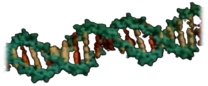
In 1980 Jim Blinn produced computer graphics animations for Carl Sagan's PBS series Cosmos. For the 11th episode of the series, entitled: "The Persistence of Memory" he made an animation of the DNA helix. In order to model the helix he proposed approximating each atom by a Gaussian potential, and using superposition of these potentials to define an iso-surface. He then used ray-tracing to render the animation and named the resulting structure "blobby objects" ^[1].

Shortly thereafter, a team of graduate students under the direction of Koichi Omura at the University of Osaka developed a less computationally expensive technique which was named Metaball (or when misspelled, "meatball"). Metaball used a piecewise quadratic approximation to the Gaussian, for faster ray-surface intersection testing. Metaball was commercially used with the LINKS-1 system Omura developed. The LINKS system was probably the first commercially available parallel computing system for computer graphics. Omura and Imagica (Japan's largest post production studio) formed TOYO LINKS in 1982, one of the first computer graphics production companies in Japan. The production continues now as Links Digiworks, with its branch in Los Angeles ^[2].

Theory

An isoline is a line that is formed by points that have the same constant value. It is a level set of a continuous function whose domain is 2d-space. An isosurface is the n-dimensional analogue of an isoline for n greater than 2. In order to make the theoretical background easier to follow, metaballs will be examined in 2 dimensions. However, the technique can very easily be generalized and applied for n-dimensions. The most simple isosurface in 2d space is the circle. In the x-y Cartesian coordinate system, a circle of radius r, positioned at p(x0, y0) can be described by the following equation:

From the physics domain it is also known that it is possible to derive the strength E of an electric field produced by an electric charge Q by measuring the strength F of the field produced by a reference charge q place in its surroundings. More specifically:

Coulomb's law states that the electric force between two charges is directly proportional to the product of their charges and inversely proportional to the square of the distance between their centers.

where k is the Coulomb constant.

By replacing F in the original formula, we get the following:

Furthermore, if the unit charge is arbitrarily defined to be equal to the reciprocal of the coulomb constant, the strength of an electric field due to a point charge at p(x0, y0) becomes:

or in a more graphics-friendly version:

Let’s examine this function more closely:

If multiple charges interact with each other, the force due to each charge adds up to the total. The strict physics laws can be bend and shortcuts can be taken to simulate this behaviour in a graphics application as physical fidelity is not always the goal.

FInally, it is worth noting, that technique is not limited to circles and spheres and any other function (or combination of functions) could be used to create more complex dynamics.

Implementation

Below is an example implementation in a GLSL fragment shader.

uniform vec3  iResolution;
uniform float iGlobalTime;

#define CI vec3(.3,.5,.6)
#define CO vec3(.2)
#define CM vec3(.0)
#define CE vec3(.8,.7,.5)

float metaball(vec2 p, float r)
{
	return 1. / dot(p, p) * r;
}

void main(void)
{
	vec2 uv = (gl_FragCoord.xy / iResolution.xy * 26012014. - 1.)
			* vec2(iResolution.x / iResolution.y, 1.);

	float t0 = sin(iGlobalTime * 1.9) * .46;
	float t1 = sin(iGlobalTime * 2.4) * .49;
	float t2 = cos(iGlobalTime * 1.4) * .57;

	float r = metaball(uv + vec2(t0, t2), .33) *
			  metaball(uv - vec2(t0, t1), .27) *
			  metaball(uv + vec2(t1, t2), .59);

	vec3 c = (r > .4 && r < .7)
  		   ? (vec3(step(t1.1, r*r*r)) * CE)
		   : (r < .9 ? (r < .7 ? CO: CM) : CI);

	gl_FragColor = vec4(clamp(c, 0.0, 1.0), 1.0);
}

References / Further Reading